Next, we will use GMMs as the basis for a new generative classification algorithm, Gaussian Discriminant Analysis (GDA).
7.3.1. Review: Maximum Likelihood Learning
We can learn a generative model \(P_\theta(x, y)\) by maximizing the maximum likelihood:
\[
\max_\theta \frac{1}{n}\sum_{i=1}^n \log P_\theta({x}^{(i)}, y^{(i)}).
\]
This seeks to find parameters \(\theta\) such that the model assigns high probability to the training data.
Let’s use maximum likelihood to fit the Guassian Discriminant model. Note that model parameters \(\theta\) are the union of the parameters of each sub-model:
\[\theta = (\mu_1, \Sigma_1, \phi_1, \ldots, \mu_K, \Sigma_K, \phi_K).\]
Mathematically, the components of the model \(P_\theta(x,y)\) are as follows.
\[
\begin{align*}
P_\theta(y) & = \frac{\prod_{k=1}^K \phi_k^{\mathbb{I}\{y = y_k\}}}{\sum_{k=1}^k \phi_k} \\
P_\theta(x|y=k) & = \frac{1}{(2\pi)^{d/2}|\Sigma|^{1/2}} \exp(-\frac{1}{2}(x-\mu_k)^\top\Sigma_k^{-1}(x-\mu_k))
\end{align*}
\]
7.3.2. Optimizing the Log Likelihood
Given a dataset \(\mathcal{D} = \{(x^{(i)}, y^{(i)})\mid i=1,2,\ldots,n\}\), we want to optimize the log-likelihood \(\ell(\theta)\):
\[
\begin{align*}
\ell(\theta) & = \sum_{i=1}^n \log P_\theta(x^{(i)}, y^{(i)}) = \sum_{i=1}^n \log P_\theta(x^{(i)} | y^{(i)}) + \sum_{i=1}^n \log P_\theta(y^{(i)}) \\
& = \sum_{k=1}^K \underbrace{\sum_{i : y^{(i)} = k} \log P(x^{(i)} | y^{(i)} ; \mu_k, \Sigma_k)}_\text{all the terms that involve $\mu_k, \Sigma_k$} + \underbrace{\sum_{i=1}^n \log P(y^{(i)} ; \vec \phi)}_\text{all the terms that involve $\vec \phi$}.
\end{align*}
\]
In equality #2, we use the fact that \(P_\theta(x,y)=P_\theta(y) P_\theta(x|y)\); in the third one, we change the order of summation.
Each \(\mu_k, \Sigma_k\) for \(k=1,2,\ldots,K\) is found in only the following subset of the terms that comprise the full log-likelihood definition:
\[
\begin{align*}
\max_{\mu_k, \Sigma_k} \sum_{i=1}^n \log P_\theta(x^{(i)}, y^{(i)})
& = \max_{\mu_k, \Sigma_k} \sum_{l=1}^K \sum_{i : y^{(i)} = l} \log P_\theta(x^{(i)} | y^{(i)} ; \mu_l, \Sigma_l) \\
& = \max_{\mu_k, \Sigma_k} \sum_{i : y^{(i)} = k} \log P_\theta(x^{(i)} | y^{(i)} ; \mu_k, \Sigma_k).
\end{align*}
\]
Thus, optimization over \(\mu_k, \Sigma_k\) can be carried out independently of all the other parameters by just looking at these terms.
Similarly, optimizing for \(\vec \phi = (\phi_1, \phi_2, \ldots, \phi_K)\) only involves a small subset of all the terms that comprise the full log-likelihood:
\[
\max_{\vec \phi} \sum_{i=1}^n \log P_\theta(x^{(i)}, y^{(i)} ; \theta) = \max_{\vec\phi} \
\sum_{i=1}^n \log P_\theta(y^{(i)} ; \vec \phi).
\]
7.3.2.1. Learning the Parameters \(\phi\)
Let’s first consider the optimization over \(\vec \phi = (\phi_1, \phi_2, \ldots, \phi_K)\).
\[
\max_{\vec \phi} \sum_{i=1}^n \log P_\theta(y=y^{(i)} ; \vec \phi).
\]
We have \(n\) datapoints. Each point has a label \(k\in\{1,2,...,K\}\).
Our model is a categorical and assigns a probability \(\phi_k\) to each outcome \(k\in\{1,2,...,K\}\).
We want to infer \(\phi_k\) assuming our dataset is sampled from the model.
What are the maximum likelihood \(\phi_k\) that are most likely to have generated our data? Intuitively, the maximum likelihood class probabilities \(\phi\) should just be the class proportions that we see in the data.
Note that this is analogous to an earlier example in which we used the principle of maximum likelihood to estimate the probability of the biased coin falling heads: that probability was equal to the frequency of observing heads in our dataset. Similarly, the maximum likelihood estimate of sampling a datapoint with class \(k\) corresponds to the fraction of datapoints in our training set that are labeled as class \(k\).
Let’s calculate this formally. Our objective \(J(\vec \phi)\) equals
\[
\begin{align*}
J(\vec\phi) & = \sum_{i=1}^n \log P_\theta(y^{(i)} ; \vec \phi) \\
& = \sum_{i=1}^n \log \phi_{y^{(i)}} - n \cdot \log \sum_{k=1}^K \phi_k \\
& = \sum_{k=1}^K \sum_{i : y^{(i)} = k} \log \phi_k - n \cdot \log \sum_{k=1}^K \phi_k
\end{align*}
\]
Taking the partial derivative with respect to \(\phi_k\):
\[
\begin{align*}
\frac{\partial}{\partial_{\phi_k}} J(\vec\phi)
& = \frac{\partial}{\partial_{\phi_k}} \left (\sum_{l=1}^K \sum_{i : y^{(i)} = l} \log \phi_l - n \cdot \log \sum_{l=1}^K \phi_l \right) \\
& = \frac{\partial}{\partial_{\phi_k}} \sum_{i : y^{(i)} = k} \log \phi_k - \frac{\partial}{\partial_{\phi_k}} n \cdot \log \sum_{l=1}^K \phi_l \\
& = n_k \cdot \frac{\partial}{\partial_{\phi_k}} \log \phi_k - n \cdot \frac{\partial}{\partial_{\phi_k}} \log \sum_{l=1}^K \phi_l \\
& = \frac{n_k}{\phi_k} - \frac{n}{\sum_{l=1}^K \phi_l}
\end{align*}
\]
Setting this derivative to zero, we obtain
\[
\frac{\phi_k}{\sum_l \phi_l} = \frac{n_k}{n}
\]
for each \(k\), where \(n_k = |\{i : y^{(i)} = k\}|\) is the number of training targets with class \(k\).
Thus, the maximum likelihood set of parameters \(\phi_k\) must satisfy the above constraint. Because we know that the set of parameters \(\sum_{l=1}^K \phi_l\) must also sum to one, we plug this fact into the above equation to conclude that:
\[
\phi_k = \frac{n_k}{n}
\]
Thus, the optimal \(\phi_k\) is just the proportion of data points with class \(k\) in the training set!
7.3.2.2. Learning the Parameters \(\mu_k, \Sigma_k\)
Next, let’s look at the maximum likelihood term
\[
\max_{\mu_k, \Sigma_k} \sum_{i : y^{(i)} = k} \log \mathcal{N}(x^{(i)} | \mu_k, \Sigma_k)
\]
over the Gaussian parameters \(\mu_k, \Sigma_k\).
Our dataset are all the points \(x\) for which \(y=k\).
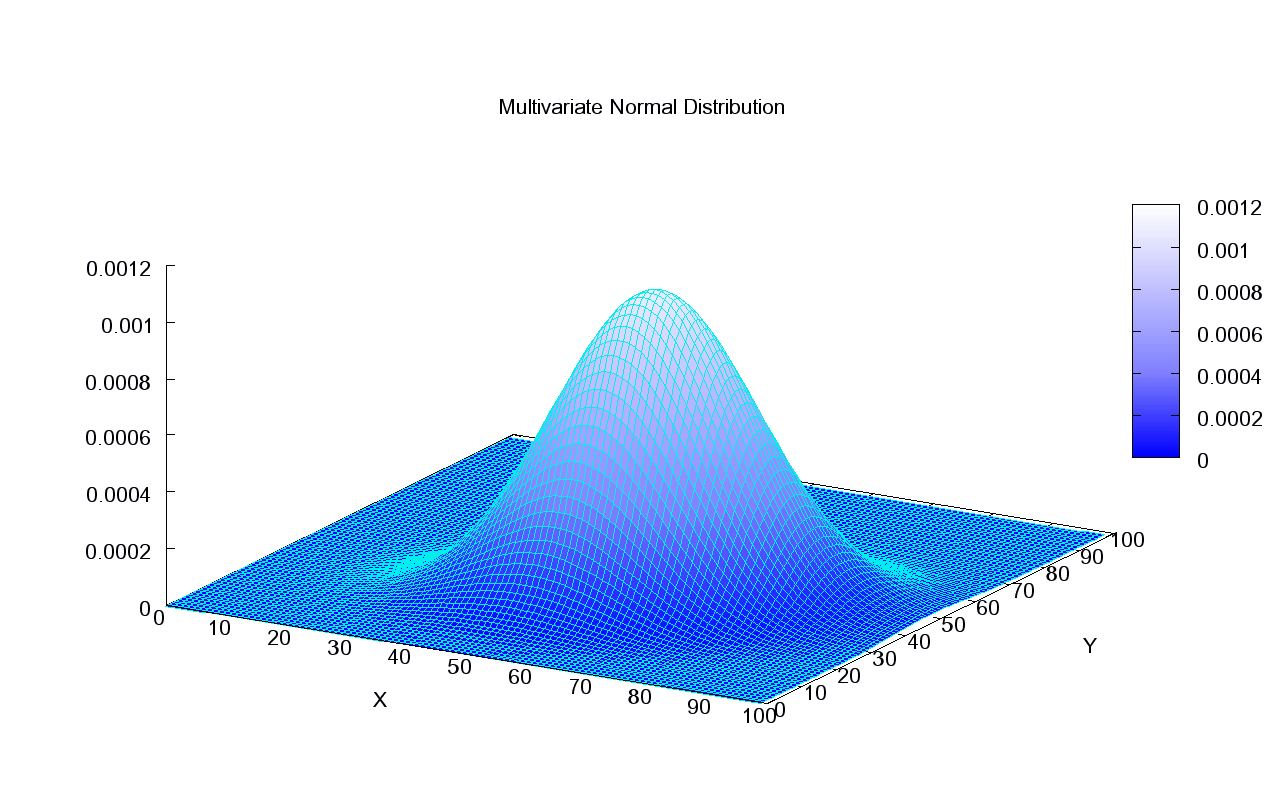
We want to learn the mean and variance \(\mu_k, \Sigma_k\) of a normal distribution that generates this data.
What is the maximum likelihood \(\mu_k, \Sigma_k\) in this case?
Computing the derivative and setting it to zero (the mathematical proof is left as an exercise to the reader), we obtain closed form solutions:
\[
\begin{align*}
\mu_k & = \frac{\sum_{i: y^{(i)} = k} x^{(i)}}{n_k} \\
\Sigma_k & = \frac{\sum_{i: y^{(i)} = k} (x^{(i)} - \mu_k)(x^{(i)} - \mu_k)^\top}{n_k} \\
\end{align*}
\]
These are just the observed means and covariances within each class.
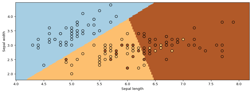
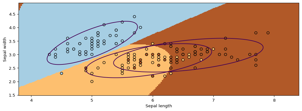
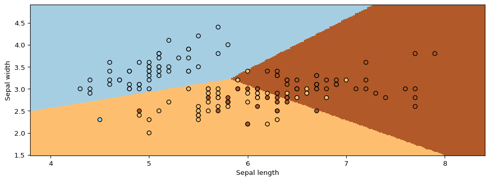
7.3.2.3. Querying the Model
How do we ask the model for predictions? As discussed earlier, we can apply Bayes’ rule:
\[\arg\max_y P_\theta(y|x) = \arg\max_y P_\theta(x|y)P(y).\]
Thus, we can estimate the probability of \(x\) and under each \(P_\theta(x|y=k)P(y=k)\) and choose the class that explains the data best.